A point/line plotting routine

Display a point/line plot of breakdowns of one or more variables.

Usage

brkdn.plot(vars,groups=NULL,obs=NULL,data,mct="mean",md="std.error",
 stagger=NULL,dispbar=TRUE,main="Breakdown plot",xlab=NULL,ylab=NULL,xaxlab=NA,
 ylim=NA,type="b",pch=1,lty=1,col=par("fg"),staxx=FALSE,yat=NULL,...)

Arguments

vars: The names or indices of one or more columns in a data frame. The columns must contain numeric data. If only one variable is to be broken down, vars can be a formula.
groups: The name or index of a column in a data frame that classifies the values in vars into different, usually fixed effect, levels.
obs: The name or index of a column in a data frame that classifies the values in vars into different, usually random effect, levels.
data: The data frame.
mct: The measure of central tendency to calculate for each group.
md: The measure of dispersion to calculate, NA for none.
stagger: The amount to offset the successive values at each horizontal position as a proportion of the width of the plot. The calculated default is usually adequate. Pass zero for none.
dispbar: Whether to display the measures of dispersion as bars.
main: The title at the top of the plot.
xlab,ylab: The labels for the X and Y axes respectively. There are defaults, but they are basic.
xaxlab: Optional labels for the horizontal axis ticks.
ylim: Optional vertical limits for the plot.
type: Whether to plot symbols, lines or both (as in plot).
pch: Symbol(s) to plot.
lty: Line type(s) to plot.
col: Color(s) for the symbols and lines.
staxx: Whether to call staxlab to display the X axis labels.
yat: Optional y axis tick positions.
...: additional arguments passed to plot.

Value

A list of two matrices of dimension length(levels(groups)) by

length(levels(obs)). The first contains the measures of central tendency calculated and its name is the name of the function passed as

mct. The second contains the measures of dispersion and its name is the name of the function passed as md.

If both groups and obs are not NULL, the rows of each matrix will be the groups and the columns the obs. If obs

is NULL, the rows will be the groups and the columns the vars. If groups is NULL, the rows will be the vars and the columns the obs. That is, if vars has more than one element, if

obs is NULL, the elements of vars will be considered to represent observations, while if groups is NULL, they will be considered to represent groups. At least one of groups and obs

must be not NULL or there is no point in using brkdn.plot.

Details

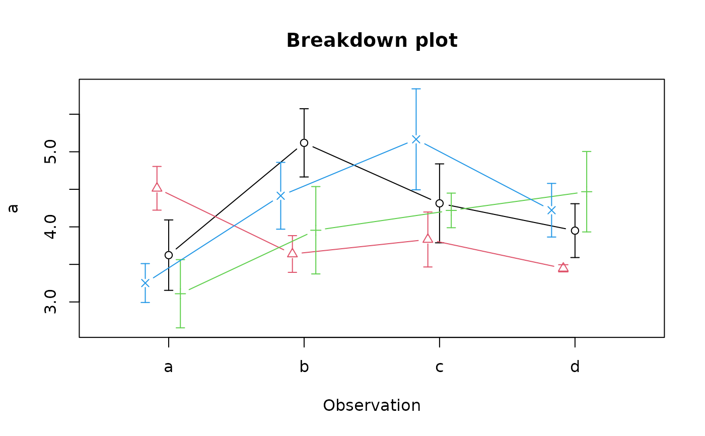
brkdn.plot displays a plot useful for visualizing the breakdown of a response measure by two factors, or more than one response measure by either a factor representing something like levels of treatment (groups) or something like repeated observations (obs). For example, if observations are made at different times on data objects that receive different treatments, the groups factor will display the measures of central tendency as points/lines with the same color, symbol and line type, while the obs factor will be represented as horizontal positions on the plot. If obs is numeric, its unique values will be used as the positions, if not, 1 to the number of unique values. This is a common way of representing changes over time intervals for experimental groups.

If only one numeric variable is to be broken down, vars may be a formula like var~groups+obs. The position of the two factors to break down the variable is fixed - the second term will be interpreted as "groups" and the third, if present, will be interpreted as "obs".

Author

Jim Lemon

Examples

 test.df<-data.frame(a=rnorm(80)+4,b=rnorm(80)+4,c=rep(LETTERS[1:4],each=20),
  d=rep(rep(letters[1:4],each=4),5))
 # first use the default values
 brkdn.plot("a","c","d",test.df,pch=1:4,col=1:4)

#> $mean
#>          [,1]     [,2]     [,3]     [,4]
#> [1,] 3.623465 5.118793 4.313158 3.949814
#> [2,] 4.513557 3.638655 3.831803 3.448280
#> [3,] 3.109367 3.954864 4.218959 4.468245
#> [4,] 3.251773 4.414033 5.165893 4.221622
#> 
#> $std.error
#>           [,1]      [,2]      [,3]       [,4]
#> [1,] 0.4688633 0.4542757 0.5256318 0.35842861
#> [2,] 0.2909573 0.2444372 0.3658918 0.04773299
#> [3,] 0.4541801 0.5816396 0.2304271 0.53571987
#> [4,] 0.2588084 0.4448299 0.6724341 0.35691044
#> 
 # now jazz it up a bit using medians and median absolute deviations
 # and some enhancements
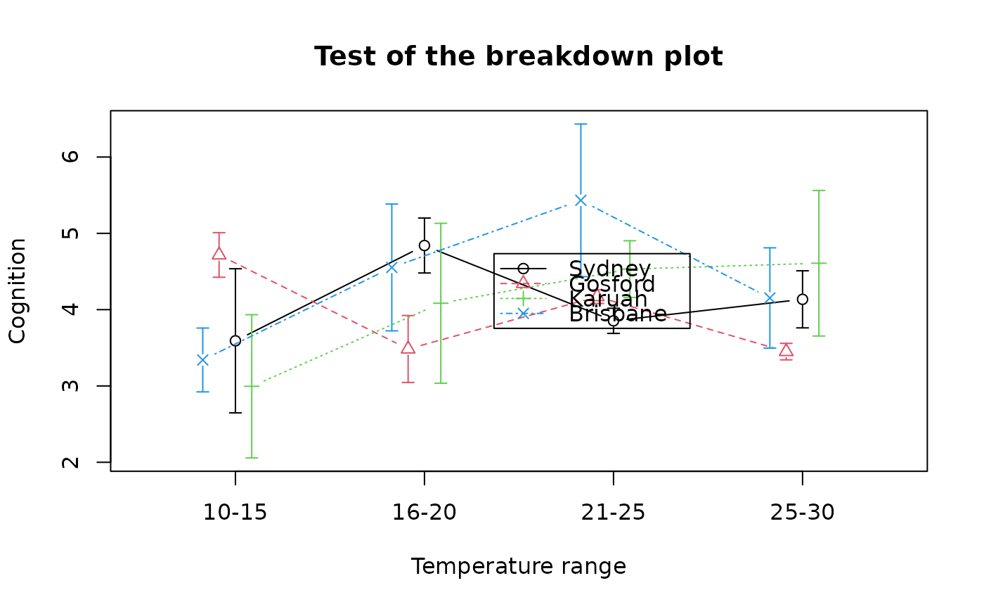
 bp<-brkdn.plot(a~c+d,data=test.df,main="Test of the breakdown plot",
  mct="median",md="mad",xlab="Temperature range", ylab="Cognition",
  xaxlab=c("10-15","16-20","21-25","25-30"),pch=1:4,lty=1:4,col=1:4)
 es<-emptyspace(bp)
 legend(es,legend=c("Sydney","Gosford","Karuah","Brisbane"),pch=1:4,
  col=1:4,lty=1:4,xjust=0.5,yjust=0.5)