raw.means.plot: Raw-Means Plots for Experimental Designs

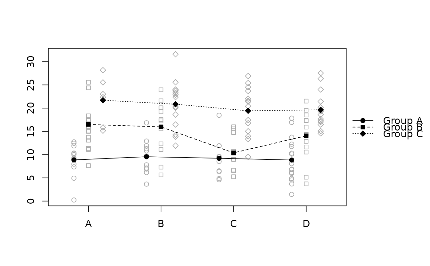
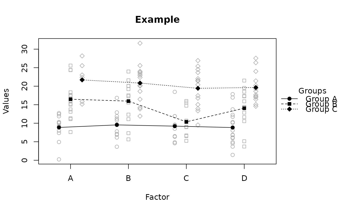
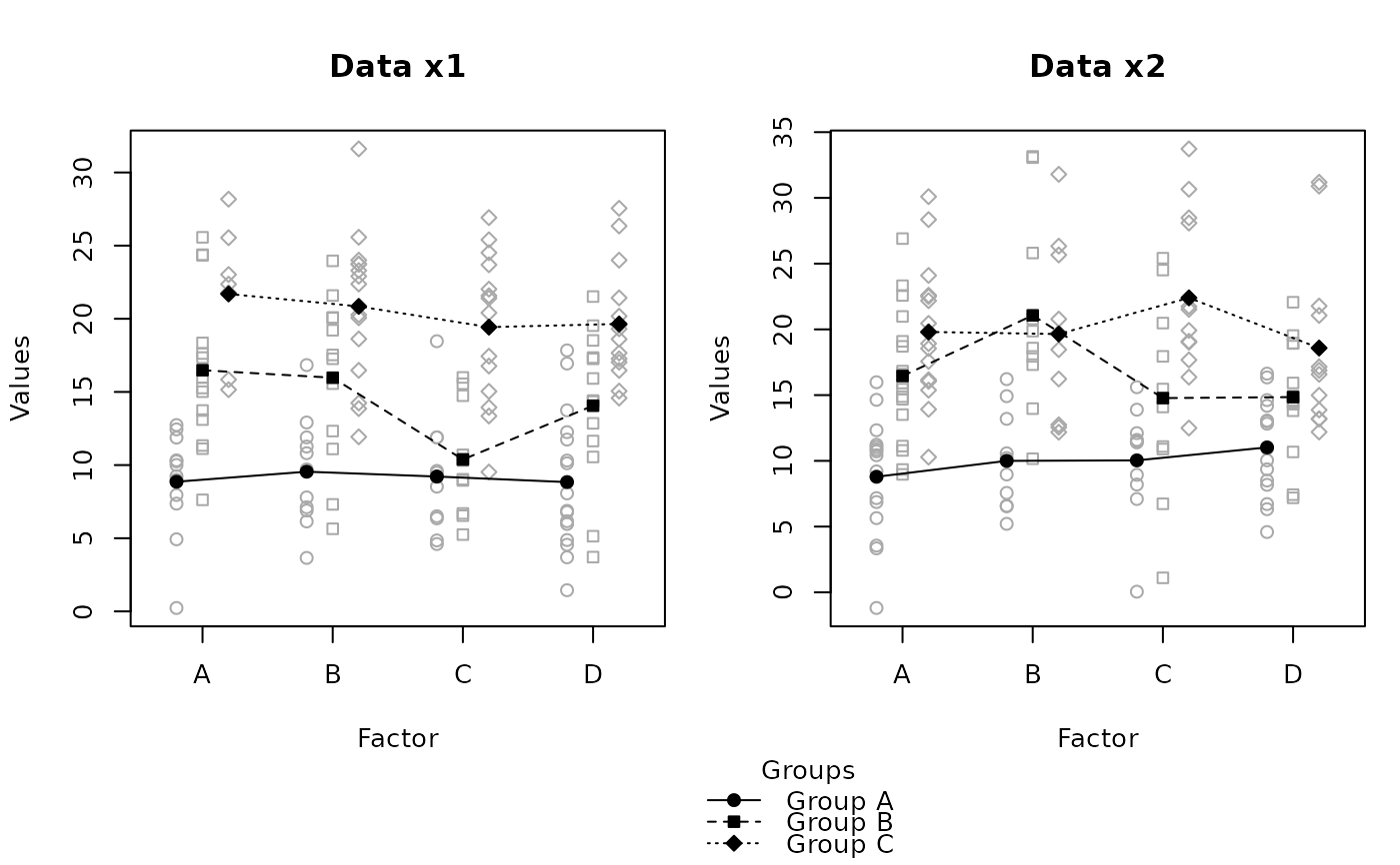
raw.means.plot is a function for visualizing results of experimental designs with up to two factors. It plots both raw data (background) and factor/cell means (foreground) to provide a more accurate visualization of the underlying distribution.

Usage

raw.means.plot(data, col.offset = 2, col.x = 3, col.value = 4, na.rm = FALSE,
 avoid.overlap = c("y", "x", "both"), y.factor = 1, y.amount = NULL,
 x.amount = 0.05, pch = 21:25, lty = 1:5, bg.b.col = "darkgrey",
 bg.f.col = NULL, fg.b.col = "black",fg.f.col = "black", type = "o",
 pt.cex = 1, lwd = 1, xlab = "", ylab = "", ylim, max.offset = 0.2,
 xaxis = TRUE, x.labels, xaxt = "n", plot = TRUE, legend = TRUE, mar = NULL,
 reset.mar = TRUE, l.pos, yjust = 0.5, l.bty = "n", l.adj = c(0, 0.5), ...)

raw.means.plot2(data, col.id, col.offset, col.x, col.value,
 fun.aggregate = "mean", ...)

Arguments

data

a data.frame in long format (i.e., each datapoint one row, see \link{reshape} or the reshape package) that contains at least three columns: one column coding the first factor (col.offset), one column coding the second factor (col.x), and one column containing the values (col.value).

col.id

a character scalar, specifiying the name of the column specifying the id column. (only for raw.means.plot2)

col.offset

a character or numeric (only raw.means.plot) scalar, specifiying either name or number of the column coding the different lines (the offset or first factor).

col.x

a character or numeric (only raw.means.plot) scalar, specifiying either name or number of the column coding the x-axis factor. Default is 3.

col.value

a character or numeric (only raw.means.plot) scalar, specifiying either name or number of the data column. Default is 4.

na.rm

logical indicating whether NA values should be stripped before the computation proceeds. Default is FALSE. Throws an error message if FALSE and NAs are encountered.

avoid.overlap

character. What should happen to datapoints within one cell of the two factors that have the same value.

"y" (the default) jitter is added so that overlapping points are distinguishable on the y-axis
"x" jitter is added so that overlapping points are distinguishable on the x-axis
"both" jitter is added so that overlapping points are distinguishable on both the y- and the x-axis.
anything else. No jitter is added.

y.factor

factor for controlling the amount of jitter on the y-axis (will be passed to jitter).

y.amount

amount for controlling the amount of jitter on the y-axis (will be passed to jitter).

x.amount

amount for controlling the amount of jitter on the x-axis (will be passed to jitter).

pch

pch values (plot symbols) taken for plotting the data. Note that the same values are taken for raw data and means. see points for more details. Recycled if too short (with warning). Default is 21:25, because those are the only values that can be displayed filled and non-filled. All other values should not be used.

lty

lty values (line types) for connecting the means. See par for more details. Recycled if too short (with warning). Default is 1:5.

bg.b.col

background border color: border color of raw data points. Silently recycled. Default: "darkgrey"

bg.f.col

background filling color: fill color of raw data points. Silently recycled. Default: NULL

fg.b.col

foreground border color: border color of mean data points. Silently recycled. Default: black

fg.f.col

foreground fill color: fill color for mean data points. Silently recycled. Default: black

type

same as type in plot. Default: o ("overplotted")

pt.cex

numeric specifying the cex value used for plotting the points. Default is 1.

lwd

numeric specifying the lwd value used for plotting the lines. Default is 1.

xlab

x-axis label. Default: ""

ylab

y-axis label. Default: ""

ylim

the y-axis limits of the plot. If not specified (the default) will be taken from data so that all raw data points are visible and a warning message is displayed specifying the ylim.

max.offset

numeric. maximal offset of factor levels from the offset factor (col.offset) specifying the different lines. The centre of each factor on the x-axis is at full numbers (starting from 1 to ...). The maximum will only be reached if the number of factor levels (from col.offset) is even. Default: 0.2.

xaxis

logical value indicating whether or not the x-axis should be generated by raw.means.plot. If TRUE, labels for the x-axis will be taken either from the unique values of col.x or can be specified with x.labels.

x.labels

character vector specifiying col.x levels. Only relevant if xaxis=TRUE. Then, the values given here will be displayed at the x-axis for each factor level of col.x.

xaxt

A character which specifies whether ot not the x-axis should be plotted by the call to plot function. Interfers with the aforementioned xaxis argument and the automatic xaxis function by raw.means.plot. Just there for completeness. Default "n" (and should not be changed).

plot

logical. Should the raw.means.plot be drawn or not. If TRUE (the default) plot will be drawn. If FALSE only the legend will be drawn (if legend = TRUE) See details.

legend

logical indicating whether or not raw.means.plot should automatically add a legend on the right outside the plot area indicating which line and points refer to which col.offset factor levels. Default is TRUE.

mar

NULL or numerical vector of length 4 indicating the margins of the plot (see par). If NULL (the default) the right margin (i.e., par("mar")[4]) will be (imperfectly) guessed from the col.offset factors for placing the legend right to the plot. If length is four this value will be taken. Ignored for plot = FALSE.

reset.mar

logical indicating if the margins (mar) shall be resetted after setting internally. Will be ignored if legend = FALSE. Default is TRUE and should not be changed (especially with plot = FLASE).

l.pos

numeric vector of length 2 indicating the position of the legend. If not specified automatically determined. See details.

yjust

how the legend is to be justified relative to the legend y location. A value of 0 means top, 0.5 means centered and 1 means bottom justified. Default is 0.5.

l.bty

the type of box to be drawn around the legend. The allowed values are "o" and "n" (the default).

l.adj

numeric of length 1 or 2; the string adjustment for legend text. Useful for y-adjustment when labels are plotmath expression. see legend and plotmath for more info.

...

further arguments which are either passed to plot or legend (or raw.means.plot for raw.means.plot2). The following arguments are passed to legend, all others are passed to plot: "fill", "border", "angle", "density", "box.lwd", "box.lty", "box.col", "pt.cex", "pt.lwd", "xjust", "x.intersp", "y.intersp", "text.width", "text.col", "merge", "trace", "plot", "ncol", "horiz", "title", "inset", "title.col", "title.adj"

fun.aggregate

Function or function name used for aggregating the data across the two factors. Default is "mean". (only for raw.means.plot2)

Details

raw.means.plot2 is probably the more useful function, as it allows for using a data.frame with more than two-factors and aggregates across the other factors, but needs a column specifying the experimental unit (e.g., participant).

raw.means.plot is basically an advanced wrapper for two other functions: plot and (if legend=TRUE) legend. Furthermore, raw data is plotted with a call to points and the means with a call to lines.

You can use raw.means.plot to plot only a legend by setting plot = FALSE and legend = TRUE. Then, raw.means.plot will draw an invisible plot with xlim = c(0,10) and ylim = c(0, 10) and place the legend on this invisible plot. You can specify l.pos to position the legend, otherwise it will be plotted at c(5,5) (i.e., in the middle of the plot). Note that xpd = TRUE in the call to legend (see par).

Value

Nothing. This function is invoked for its side effects.

Author

Henrik Singmann (henrik.singmann@psychologie.uni-freiburg.de) with ideas from Jim Lemon

Examples


x <- data.frame(id = 1:150, offset = rep(c("Group A", "Group B", "Group C"),
 each = 50), xaxis = sample(c("A", "B", "C", "D"),150, replace = TRUE),
 data = c(rnorm(50, 10, 5), rnorm(50, 15,6), rnorm(50, 20, 5)))

raw.means.plot(x)
#> Warning: Converting offset variable (column 2) to factor.
#> Warning: Converting x-axis variable (column 2) to factor.
#> Warning: ylim not specified, taken from data: 0.232797172609803 - 31.6117451952093


raw.means.plot(x, main = "Example", ylab = "Values", xlab = "Factor",
 title = "Groups")
#> Warning: Converting offset variable (column 2) to factor.
#> Warning: Converting x-axis variable (column 2) to factor.
#> Warning: ylim not specified, taken from data: 0.232797172609803 - 31.6117451952093


raw.means.plot(x, "offset", "xaxis", "data")
#> Warning: Converting offset variable (column offset) to factor.
#> Warning: Converting x-axis variable (column offset) to factor.
#> Warning: ylim not specified, taken from data: 0.232797172609803 - 31.6117451952093


raw.means.plot(x, "xaxis", "offset", "data")
#> Warning: Converting offset variable (column xaxis) to factor.
#> Warning: Converting x-axis variable (column xaxis) to factor.
#> Warning: ylim not specified, taken from data: 0.232797172609803 - 31.6117451952093

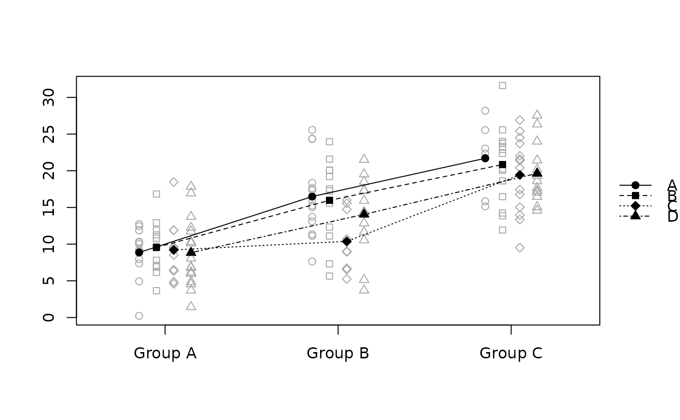raw.means.plot(x, 3, 2, 4)
#> Warning: Converting offset variable (column 3) to factor.
#> Warning: Converting x-axis variable (column 3) to factor.
#> Warning: ylim not specified, taken from data: 0.232797172609803 - 31.6117451952093


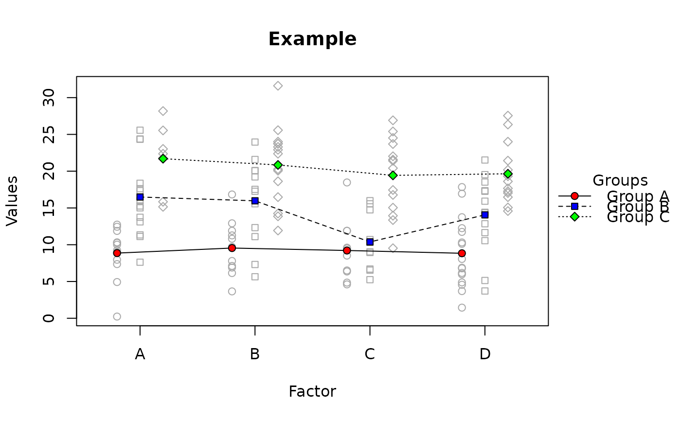
# different colors:
raw.means.plot(x, main = "Example", ylab = "Values", xlab = "Factor",
 title = "Groups", fg.f.col = c("red","blue", "green"))
#> Warning: Converting offset variable (column 2) to factor.
#> Warning: Converting x-axis variable (column 2) to factor.
#> Warning: ylim not specified, taken from data: 0.232797172609803 - 31.6117451952093


x2 <- data.frame(id = 1:150, offset = rep(c("Group A", "Group B", "Group C"),
 each = 50), xaxis = sample(c("A", "B", "C", "D"),150, replace = TRUE),
 data = c(rnorm(50, 10, 5), rnorm(50, 15,6), rnorm(50, 20, 5)))

layout(matrix(c(1,2,3,3), 2,2,byrow = TRUE), heights = c(7,1))
raw.means.plot(x, main = "Data x1", ylab = "Values", xlab = "Factor",
 legend = FALSE, mar = c(4,4,4,1)+0.1)
#> Warning: Converting offset variable (column 2) to factor.
#> Warning: Converting x-axis variable (column 2) to factor.
#> Warning: ylim not specified, taken from data: 0.232797172609803 - 31.6117451952093
raw.means.plot(x2, main = "Data x2", ylab = "Values", xlab = "Factor",
 legend = FALSE, mar = c(4,4,4,1)+0.1)
#> Warning: Converting offset variable (column 2) to factor.
#> Warning: Converting x-axis variable (column 2) to factor.
#> Warning: ylim not specified, taken from data: -1.1902265035568 - 33.7265689930563
raw.means.plot(x2, plot = FALSE, title = "Groups")
#> Warning: Converting offset variable (column 2) to factor.
#> Warning: Converting x-axis variable (column 2) to factor.
#> Warning: ylim not specified, taken from data: -1.1902265035568 - 33.7265689930563



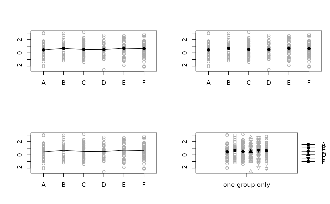
y <- data.frame(id = 1:300, offset = rep(1, 300),
 axis = sample(LETTERS[1:6],300, replace = TRUE), data = c(rnorm(100, 1),
 rnorm(100), rnorm(100,1)))

par(mfrow = c(2,2))

raw.means.plot(y, legend = FALSE)
#> Warning: Converting offset variable (column 2) to factor.
#> Warning: Converting x-axis variable (column 2) to factor.
#> Warning: ylim not specified, taken from data: -2.5500144848278 - 3.11278759570127

raw.means.plot(y, type = "p", legend = FALSE)
#> Warning: Converting offset variable (column 2) to factor.
#> Warning: Converting x-axis variable (column 2) to factor.
#> Warning: ylim not specified, taken from data: -2.5500144848278 - 3.11278759570127

raw.means.plot(y, type = "l", legend = FALSE)
#> Warning: Converting offset variable (column 2) to factor.
#> Warning: Converting x-axis variable (column 2) to factor.
#> Warning: ylim not specified, taken from data: -2.5500144848278 - 3.11278759570127

raw.means.plot(y, 3, 2, x.labels = "one group only")
#> Warning: Converting offset variable (column 3) to factor.
#> Warning: Converting x-axis variable (column 3) to factor.
#> Warning: ylim not specified, taken from data: -2.5500144848278 - 3.11278759570127
#> Warning: pch vector too short. recycling pch vector.
#> Warning: lty vector too short. recycling lty vector.



# Example with overlapping points
z <- data.frame (id = 1:200, offset = rep(c("C 1", "C 2"), 200),
 axis = sample(LETTERS[1:4], 200, replace = TRUE),
 data = sample(1:20, 200, replace = TRUE))

# x versus y jitter
par(mfrow = c(2,2))
raw.means.plot(z, avoid.overlap = "none", main = "no-jitter")
#> Warning: Converting offset variable (column 2) to factor.
#> Warning: Converting x-axis variable (column 2) to factor.
#> Warning: ylim not specified, taken from data: 1 - 20
raw.means.plot(z, main = "y-axis jitter (default)")
#> Warning: Converting offset variable (column 2) to factor.
#> Warning: Converting x-axis variable (column 2) to factor.
#> Warning: ylim not specified, taken from data: 1 - 20
raw.means.plot(z, avoid.overlap = "x", main = "x-axis jitter")
#> Warning: Converting offset variable (column 2) to factor.
#> Warning: Converting x-axis variable (column 2) to factor.
#> Warning: ylim not specified, taken from data: 1 - 20
raw.means.plot(z, avoid.overlap = "both", main = "both-axis jitter")
#> Warning: Converting offset variable (column 2) to factor.
#> Warning: Converting x-axis variable (column 2) to factor.
#> Warning: ylim not specified, taken from data: 1 - 20



# y-axis jitter (default)
par(mfrow = c(2,2))
raw.means.plot(z, avoid.overlap = "none", main = "no jitter")
#> Warning: Converting offset variable (column 2) to factor.
#> Warning: Converting x-axis variable (column 2) to factor.
#> Warning: ylim not specified, taken from data: 1 - 20
raw.means.plot(z, y.factor = 0.5, main = "smaller y-jitter")
#> Warning: Converting offset variable (column 2) to factor.
#> Warning: Converting x-axis variable (column 2) to factor.
#> Warning: ylim not specified, taken from data: 1 - 20
raw.means.plot(z, main = "standard y-jitter")
#> Warning: Converting offset variable (column 2) to factor.
#> Warning: Converting x-axis variable (column 2) to factor.
#> Warning: ylim not specified, taken from data: 1 - 20
raw.means.plot(z, y.factor = 2, main = "bigger y-jitter")
#> Warning: Converting offset variable (column 2) to factor.
#> Warning: Converting x-axis variable (column 2) to factor.
#> Warning: ylim not specified, taken from data: 1 - 20



# x-axis jitter (default)
par(mfrow = c(2,2))
raw.means.plot(z, avoid.overlap = "none", main = "no jitter")
#> Warning: Converting offset variable (column 2) to factor.
#> Warning: Converting x-axis variable (column 2) to factor.
#> Warning: ylim not specified, taken from data: 1 - 20
raw.means.plot(z, avoid.overlap = "x", x.amount = 0.025,
 main = "smaller x -jitter")
#> Warning: Converting offset variable (column 2) to factor.
#> Warning: Converting x-axis variable (column 2) to factor.
#> Warning: ylim not specified, taken from data: 1 - 20
raw.means.plot(z, avoid.overlap = "x", main = "standard x-jitter")
#> Warning: Converting offset variable (column 2) to factor.
#> Warning: Converting x-axis variable (column 2) to factor.
#> Warning: ylim not specified, taken from data: 1 - 20
raw.means.plot(z, avoid.overlap = "x", x.amount= 0.1,
 main = "bigger x-jitter")
#> Warning: Converting offset variable (column 2) to factor.
#> Warning: Converting x-axis variable (column 2) to factor.
#> Warning: ylim not specified, taken from data: 1 - 20




if (FALSE) {

#The examples uses the OBrienKaiser dataset from car and needs reshape.
require(reshape)
require(car)
data(OBrienKaiser)
OBKnew <- cbind(factor(1:nrow(OBrienKaiser)), OBrienKaiser)
colnames(OBKnew)[1] <- "id"
OBK.long <- melt(OBKnew)
OBK.long[, c("measurement", "time")] <-
 t(vapply(strsplit(as.character(OBK.long$variable), "\\."),  "[", c("", "")))

raw.means.plot2(OBK.long, "id", "measurement", "gender", "value")

raw.means.plot2(OBK.long, "id", "treatment", "gender", "value")

# also use add.ps:
# For this example the position at each x-axis are within-subject comparisons!
raw.means.plot2(OBK.long, "id", "measurement", "gender", "value")
add.ps(OBK.long, "id", "measurement", "gender", "value", paired = TRUE)
 #reference is "fup"

raw.means.plot2(OBK.long, "id", "measurement", "gender", "value")
add.ps(OBK.long, "id", "measurement", "gender", "value", ref.offset = 2,
 paired = TRUE) #reference is "post"

# Use R's standard (i.e., Welch test)
raw.means.plot2(OBK.long, "id", "treatment", "gender", "value")
add.ps(OBK.long, "id", "treatment", "gender", "value",
 prefixes = c("p(control vs. A)", "p(control vs. B)"))

# Use standard t-test
raw.means.plot2(OBK.long, "id", "treatment", "gender", "value")
add.ps(OBK.long, "id", "treatment", "gender", "value", var.equal = TRUE,
 prefixes = c("p(control vs. A)", "p(control vs. B)"))

}